计算几何 W48 Robot Motion Planning and Visibility (新课完结)
Robot Motion Planning
Given a set of obstacles , and a polygonal robot with starting configuration and target configuration . Find a path for the robot from to if possible.
机器人路径规划问题,首先应该先解决:存不存在这样一条路径的问题。
Reference point
define a reference point of the robot and define position of the vertices of w.r.t. .
Suppose our robot can move by translating
: position of the robot when the reference point is at .
Suppose our robot can move by translating:
: position of the robot when the reference point is at and the robot has orientation .
We represent the robot by a point in the parameter space (configuration space)
先只考虑机器人只能平移,不能旋转。
partition the configuration space in free space and forbidden space
in forbidden space intersects an obstacle.
can move from to there is a path from to in the free space.
对于机器人上的一个参考点,在图上都有一个 free space 图。如果 free space 联通起始点,那么就存在一个路径使得机器人可以从起点移动到终点。
if is a point then configuration space = work space.
Finding a path in the Configuration Space
如果存在路径,那么就找出这样一条路径
given a configuration space of complexity find a path from to if possible.
idea: construct a trapezoidal decomposition of the free space.
思路:将 free space 用竖线进行梯形分解。
construct a road map
: set of all centers of all trapezoids and all midpoints of all vertical segments .
梯形的中位线中点+所有梯形顶边和底边线段的中点
is a vertical segment bounding .
add and to and connect them to the trapezoids containing them.
Run a BFS in the road map to find a path from to .
Theorem
we can compute a path from to in expected time.
如何搞定 free space 的计算问题呢?使用闵可夫斯基和解决!
Minkowski Sums
Let and be two sets in
P\oplus R=\{p+r|p\in R\and r\in R\} is the Minkowski sum of and .
where
observation: let , an extreme point on in direction is the sum of extreme points in direction on and .
Theorem
- Let and be convex polygons with and edges, then is a convex polygon and has at most edges.
- Let and be convex polygons with and edges, then can e computed in time.
Question: What if and are not convex?
Pseudo-discs
a pair and are pseudo-discs
the boundaries of and intersect in at most two points.
i.e.,
observation: A pair of polygonal pseudo-discs and defines at most two boundary crossing
Theorem
Let be a collection of convex polygonal pseudo-discs with a total of edges. the total complexity of their union is at most .
- pseudo-disk vertices
- intersection points
Charge every pseudo-disk vertex to itself.
For an intersection point , by observation: either
- has no other boundary crossing with \part R.
- has no other boundary crossing with \part P, or both
Let be the edge without other boundary crossings, and let be the endpoint of in .
Charge to .
Claim: Every vertex (of a pseudo-disk ) is charged at most twice.
Case 1: not in any other pseudo-disk ∴ is a green vertex and is charged only by itself.
Case 2: lies in the interior of the union.
Traverse . There is only one point on the boundary of the union on that charges to .
Same for the other edge
Case 3: v,v\in\part R lies on the boundary of the union. As in case 2 is charged only by its incident edges and and by itself
can not be charged by both its incident edges at the same time.
Let be a collection of pseudo-discs with a total of edges. The total complexity of their union is at most .
Observation: Let and be convex polygons with disjoint interiors, let and be directions where is more extreme than .
Then either
- is more extreme in all directions in , or
- is more extreme in all directions in .
Let and be two convex polygons with disjoint interiors, and let be another convex polygon. Then and are pseudo-discs.
To show: \part P\oplus R\cap int(Q\oplus R) is connected.
Proof by contradiction. Assume \part P\oplus R\cap int(Q\oplus R) is not connected.
By observation, an extreme point on corresponds to a extreme point on . Same for .
more extreme on and than
more extreme on and than
What if is not convex?
observation: for any set
Triangulate
this produces a collection of disjoint convex polygons, so the collection of Minkowski sums is a collection of pseudo-disks.
Let be a polygon with vertices, and let be a convex polygon with vertices. Then complexity of is .
What if and are both not convex?
Triangulate both and . This gives a collection of triangles.
Let be a polygon with vertices, and let be a convex polygon with vertices, The complexity of is .
Let be a polygon with vertices, and let be a convex polygon with vertices, we can compute in time.
好麻啊这一段
Minkowski Sum & Robot Motion Planning
Let and
Lemma. Let be an obstacle and let be a planar, translating robot. A point in the configuration space is forbidden iff .
In direction:
suppose
Only if direction: similar.
Question: How do we compute the free/forbidden space in the configuration space?
Forbidden space
So if is convex and has constant complexity, and the input polygons have a total vertices we can compute the forbidden space in time.
Shortest Paths
Given a set of obstacles , a starting point and target point . Find a shortest path from to ,
Lemma A shortest pat between and among a st of disjoint obstacles is a polygonal path whose inner vertices are vertices of .
Question: how do we compute a shortest path between and ?
idea: Construct a graph with edge length s.t. for the edge corresponds to the distance between and .
the set of obstacle vertex and and
and can see each other
Theorem: We can compute in time.
Visibility Graph
Connecting two vertices if they can see each other.
Sub-goal: compute all visible vertices from any point in time.
i.e. visibility graph in time.
Idea: Radical sweep ray!
Exactly identical to normal sweep line, if we rotate the ball until is a point at infinity.
我的理解是把这个看成以该点为极点的极坐标,可以映射到一个以该点为原点的直角坐标。就可以转化为最普通的扫描线了。
Find vertices visible from X-coordinate.
Compute visible vertices from to , add to visibility graph, then use Dijkstra for time in total.
(can be improved to )