数据挖掘 6 Spectral Theory and Clustering
This module introduces graph mining.
Data points from networks, graphs, of connections.
Purpose: extract patterns from graphs.
3 different areas of graph mining:
- Community detection: finding groups of nodes with similar characteristics.
- Link analysis: understanding which node is more important than others.
- Embedding: capturing similarities among nodes.
Graph : a set of vertices connected through edges .
undirected & directed graph
Graph representations. A graph can be represented by adjacency lists or an adjacency matrix.
Degree of a node.
Graph construction:
- KNN graph: connect every point with its closest points.
- -neighborhood: connect all points with the points within distance.
- Fully-connected graph: choose a distance , then connect any point to any other point. The weight of each edge corresponds to between and .
The Adjacency Matrix
Consider undirected graphs. Their adjacency matrix is symmetric.
By multiplying a vector with a adjacency matrix.
can be thought as the vector form of a function .
The vector ’s -th element is . Therefore, the entry is the sum of labels of neighbors of . This means that is a matrix that transforms the value of a node as a sum of the value of the neighbors. If we repeat this aggregation multiple times we obtain a propagation of the initial labels over the network
There exists a fixed-point in this iteration:
We want to find an eigenvector and eigenvalue for the matrix .
Spectral Graph Theory
Analyzing properties of the graph by inspecting the eigenvalues and eigenvectors of matrices that represent the graph structure.
Given a graph and a matrix that describes the graph’s structure, the graph spectrum is the set of ’s eigenvalues sorted in descending order
is an eigenvalue if there exists a vector s.t. \mathbf{Ax}=\lambda\mathbf x\Lrarr(\mathbf A-\lambda\mathbf I)\mathbf x=0\Rarr\mathbf\det(A-\lambda\mathbf I)=0
For symmetric matrices. is symmetric, This means . Thus,
All eigenvalues are positive
The matrix is positive semi-definite, .
matrix , s.t.
All eigenvalues are real numbers, all eigenvectors are orthogonal ().
In a -regular graph, that is an eigenvector. That means all the eigenvectors should be . This is a very important fact that will be used later.
A graph is -regular, if the degree for every vertex is .
Graph Matrices
The degree matrix denoted is an diagonal matrix where is the degree of node .
Unnormalized Laplacian Matrix or is an matrix.
Normalized Symmetric Laplacian or is the normalized version of .
Asymmetric (Random Walk) Laplacian or .
Laplacian’s properties: It has a trivial eigenvector corresponding with the eigenvalue since . Moreover, Laplacian is symmetric and positive semi-definite, all the eigenvalues are non-negative real numbers and the eigenvectors are real and orthogonal.
Spectral Clustering
A cut is a set of edges with only one vertex in a group
If we directly minimize the cut we might end up in unfortunate solution in which a partition contains only one node. To avoid this, we can minimize a normalized cut
Where . Computing optimal normalized cuts is NP-hard.
Another approach to write the cut is considering a variable for each vertex , s.t.
Thus .
So if we want to minimize the cut we can just minimize the sum of absolute differences among entries. It’s more convenient instead to minimize . However, as we have seen this corresponds to .
Similarly, we can see that
corresponds to a normalized version of the cut and is called the Rayleigh quotient. (瑞利商)
Minimum-cut Relates to Spectral Properties
Variantional characterization of eigenvalues. Consider a matrix real and symmetric. The eigenvalues are sorted in decreasing order. The variational characterization of the eigenvalues states that states that the smallest eigenvalue corresponds to
where is the eigenvector corresponding to the eigenvalue . Similarily, the second smallest eigenvector is the solution
And so on with all the eigenvalues. Finally,
Minimum cut as eigenvalues of the Laplacian.
- All eigenvectors a symmetric matrix are orthogonal and that the Laplacian matrix for an undirected graph is a symmetric matrix.
- The eigenvalue that minimizes is the eigenvalue that corresponds to the eigenvector of the graph’s Laplacian . This corresponds to placing all nodes into a single partition.
- The second smallest corresponds to an eigenvector , which is orthogonal to the eigenvector , i.e. .
- The eigenvector is called the Fiedler’s vector and minimizes a relaxed version of the normalized cut.
Spectral Clustering Algorithm
Spectral clustering works in 3 phases:
- Preprocessing: Construct a matrix representation of the graph.
- Decomposition: compute the eigenvalues and eigenvectors of the matrix. Map each point to a lower-dimensional representation based on one or more eigenvectors.
- Grouping: Assign points to two or more clusters, based on the new representation.
The Spectral Partitioning Algorithm finds a partition of the graph that is close to the optimal partition. In the decomposition phase, Spectral clustering maps vertices to corresponding components of and its vector. In the grouping phase, we sort the components of the new 1-dimensional vector and split then nodes in positive and negative or using the median value.
-way Spectral Clustering
We extend spectral clustering to the case of finding -partitions.
One strategy is to recursively split the graphs into two partitions, until partitions are returned.
Another strategy leverages multiple eigenvectors besides the one corresponding to the second smallest eigenvalue. By stacking on the eigenvectors each node is embedded into a multi-dimensional space. Finally, we run -means in this new space to find -partitions.
Advantages of using multiple eigenvectors:
- Approximates the optimal cut
- Emphasizes cohesive clusters by increasing the unevenness in the distribution in the data.
- Provides a well-separated space. It transforms data to a new embedded space consisting of orthogonal basis vectors.
- Multiple eigenvectors prevent instability caused by information loss.
Pros and Cons
👍
- Clusters can have arbitrary shapes and size and are not restricted to convex shapes.
- Efficient in normal space graphs.
- Robust to noise is theoretically grounded and well-connected to graph properties.
👎
- Inefficient on dense graph - worst case.
- Need to provide number of clusters .


